ADRENALIN 2023: Smart building HVAC control challenge

Background

Buildings account for a significant portion of global energy consumption, the bulk of it for heating and cooling, and reducing energy use in buildings is critical to meeting global emissions reduction targets.  

With introduction of more renewables and electrification of heating systems and the mobility sector, the strain on the energy grids is drastically increased. However, buildings also have a large potential for flexibility thanks to their slow thermal inertia. Consequently, buildings offer the potential to be one of the lowest cost opportunities for providing the flexible demand needed to support increasing levels of variable renewable energy resources in electricity grids. 

To release this flexibility potential, smart control algorithms, that can respond to external signals, such as price variations, are needed. However, implementation of smart control algorithms in buildings are a time consuming and costly task. Evaluation of control algorithms in a simplified virtual environment to identify the most promising concepts are needed. 

The Smart building HVAC control challenge aims to develop efficient and scalable control algorithms that can be applied in commercial buildings to reduce energy consumption and release their flexibility potential. 

Problem statement

The development and implantation of smart control algorithms is a complex task that requires development of scalable, transferable and efficient solutions. This competition seeks to address this challenge by promoting development and benchmarking of various control strategy approaches, that are applicable for implementation in real buildings. 

The competition will challenge participants to develop scalable, efficient, and effective algorithms that can release the flexibility potential in building HVAC systems, while taking the following key challenges into account:

• Activation of flexibility: The challenge will focus on controllers ability to activate the building HVAC system’s flexibility potential based on variable cost signals, while not compromising indoor air quality.

• Scalability: Many smart control algorithms require a lot of individual adaption for implementation in different buildings. This is time and cost intensive, and makes it less profitable to install. The competition will promote solutions that are scalable from an implementation perspective.

Participation and Submission

I     Register at the Adrenalin competition dashboard (Codalab)

1. To register a Codalab account go to https://codalab.lisn.upsaclay.fr/accounts/signup

2. Go to the competition’s page: (link will be available at a later date)
3. Navigate to the “Participate” tab to accept the terms and conditions and register for the competition.

II    Run and train your controller

In the training phase of the competition, the testcases can be run both locally and through the BOPTEST service.

How to run the testscase locally:

1. Download the testcase FMUs from here: link
2. Download BOPTEST from here: https://github.com/ibpsa/project1-boptest/releases/tag/v0.5.0

Or clone directly from GitHub.Make sure to checkout commit “v0.5.0”

1. Inside the BOPTEST/testcases folder. Create a new testcase with the name of the testcase
2. Load BOPTEST using docker compose and the testcase name, as described here: https://github.com/ibpsa/project1-boptest
3. Follow the steps shown in the attached jupyter notebook. More detailed information on the BOPTEST API can be found at the BOPTEST repository: https://github.com/ibpsa/project1-boptest

Run with service version:

1. Follow the instructions in the Jupiter notebook. More details on the service specific API are given here: https://github.com/NREL/boptest-service

III   Submit your results to the competition dashboard

For a result to be valid for submission to the competition, it must be ran through the BOPTEST service.  

Submission is done by submitting the test_id retrieved from the BOPTEST service.

The test_id is retrieved when initializing a testcase from the BOPTEST service, with:

POST testcases/{namespace}/{testcase_name}/select

Make sure the testcase is run until finished before submitting the test_id to the Adrenalin dashboard. You should create and submit different test_id’s for each scenario and testcase.

To make a submission, a zipped csv file has to be uploaded on Codalab. The csv file must contain 4 rows and two columns. One row for each scenario and testcase. The first column is the identifier, and the second column is for the test_id retrieved from the BOPTEST service. If some test_ids are left blank, only the submitted scenarios are scored. A submission template is provided here: (Link will be available at a later date)

The test_ids are submitted through the competition dashboard. The submission score is calculated in the back-end and displayed on the dashboard.

Evaluation Criteria

The evaluation will be two-folded.

1. Quantitative evaluation based on KPIs in the BOPTEST framework. A single number will be calculated based weighting of the different KPIs. See further description below
2. Qualitative evaluation taking into account the complexity of the control, data requirement and scalability. As part of the submission, the participant will be asked to document their control algorithm.

The prize money will be distributed evenly on the two evaluation parts.

For the 3 best scoring contributions for the quantitative evaluation will be distributed accordingly:

1. XXX€
2. XX€
3. X€

Those three contributions will then be reevaluated through the qualitative evaluation.

Quantitative evaluation

The quantitative evaluation will be using a selection of the standard KPIs from the BOPTEST framework, and weighting them in a total score. The descriptions of the relevant KPIs are shown in the table below.

Table 1: KPIs

The score of a controller on a single scenario (i) is given by the following equation:

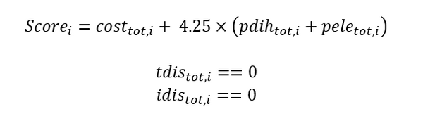
The score equation contains energy cost plus a peak power penalty, representing a peak power tariff. The energy prices for electricity and district heating are the same and are based on electricity spot prices for the location of the building. However, as an important factor in the competition, is for the controller to demonstrate its ability to exploit the flexibility of the building, the spot price signal is exaggerated. The baseline controllers are price ignorant.

The discomfort KPIs (thermal and IAQ) are handled as hard constraints. For the result to be valid, the discomfort constraints should not be violated. The baseline controller is designed with a margin, to make sure that the baseline does not violate the comfort constraints, and give a possibility for improvement.

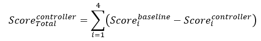
The total score of a submission will be the sum of the difference between the score of the baseline controller and submission controller for all scenarios:

For a submission to be eligible for the prize money, the score for each scenario must be positive.

Qualitative evaluation

In addition to submission of the controller performance, the participants must fill out a template describing their control approach.

The qualitative evaluation will focus on the prospect of application in real buildings. Important points are

• Model complexity
• Training data demand
• Interpretability (How well can the decisions be understood by users?)

The 3 best contributions from the quantitative evaluation will be invited to a Q&A session, where they must present their solution and answer questions from the evaluation committee.

After the Q&A session the committee will distribute the price money as they wish.

Timeline

•  Training stage (phase I)

The training period will last for 2 months. In this period, the participants will get access to a training version of each of the emulators. The emulators will be available through the BOPTEST service and for download to run it locally. More information on how to install and run the emulators is given in section Emulators.

The participants can use this period to train and test their control algorithms. It is however encouraged that participants submit their intermediate results from the training to the competition dashboard (Participation and Submission).

To continue to the competition stage, a full, valid result (for both emulators and scenarios) must be run with the BOPTEST service version and submitted to the Adrenalin dashboard.

• Competition stage (Phase II)

The competition stage will last 5 days. For this stage, new versions of the emulators (same emulators but slightly different boundary conditions) will be made available. The emulators will be available only through the service version of BOPTEST. To be eligible for the prize money valid results for both scenarios in both emulators must be submitted to the Adrenalin dashboard.

Prizes

Coming Soon!

Emulators

The competition will be performed using the BOPTEST framework (https://ibpsa.github.io/project1-boptest/).

Each of the emulators have two scenarios defined each: “typical_heat_day” and “peak_heat_day”. These represent periods with typical heat demand and peak heat demand respectively. For energy prices, only the “highly_dynamic” scenario will be used in the competition evaluation.

Emulator 1: Single zone commercial hydronic

General description

This emulator is based on the BOPTEST Single zone commercial hydronic emulator developed by the University of Southern Denmark (SDU). Detailed description of the original emulator can be found here: https://ibpsa.github.io/project1-boptest/docs-testcases/singlezone_commercial_hydronic/index.html

This chapter describes where the Adrenalin emulator differs from the original BOPTEST emulator.

Architecture and construction

The architecture and construction of the building is equal to the original BOPTEST emulator.

Occupancy and internal gains

The occupancy profile is based on the collected data described for the original emulator, with some small changes. Internal heat gains of 120 W/person are added to the thermal zone, radiative (40%), convective (40%), and latent gains (20%). The internal gains from electrical equipment and lighting is estimated to be part of this, but is not measured separately.

HVAC

Ventilation

The layout of the ventilation system is similar to the original BOPTEST emulator, but the performance characteristics and control of some of the components are different.

Figure 1 shows a principle flow sheet for the air handling unit (AHU), as modeled in the emulator. It shows the placement of the sensors and components and the control principle.

• The supply fan relative speed (0-1) is controlled by the CO₂ level in the building. Minimum relative fan speed is set to 30 % in the baseline control.
• The extract fan relative speed (0-1) is controlled by the supply air flow rate, to keep equal supply and extract flow. Minimum relative fan speed is set to 20 % in the baseline control.
• The speed of the rotary wheel in the heat recovery unit is controlled to try to reach the supply temperature set point temperature.
• The valve on the hydronic heating battery is controlled to reach the supply temperature setpoint temperature.

Figure 2 shows the fan characteristics. The grey line shows the operational point at nominal speed.

Figure 1: Principle ventilation flow sheet

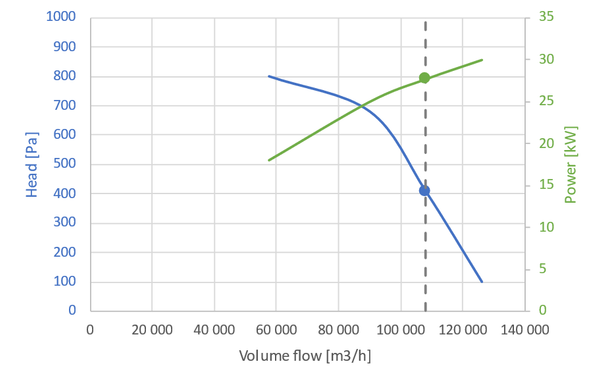
Figure 2: Fan characteristics

Hydronic heating system

The layout of the hydronic heating system is shown in Figure 3. Piping segments are modeled between the main distribution pipes and the control valves for both the ventilation and radiator circuits.

Heat is supplied by a district heating system. The temperature of the district heating is fixed to 65 °C. The supply temperature of the hydronic heating system is controlled by the flow on the primary side of the district heating heat exchanger. The setpoint follows the outdoor temperature compensation curve shown in Figure 4.

The main circulation pump sustains a fixed pressure across the distribution pipes. The baseline setpoint is 50 000 Pa. This is also the maximum possible pressure difference of the pump.

The control valve of the radiator tracks the measured indoor temperature. The baseline controller implements a night setback of 3 K outside of operating hours. After night setback, the setpoint is reset to 22 °C 2 hours before the next operating hour (4 hours on Mondays), to make sure the building has reached the setpoint temperature before the building is occupied again.

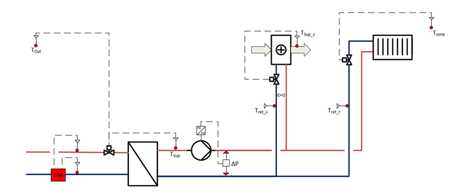
Figure 3: Principle hydronic flow sheet

The design specifications of the heat exchangers are given in Table 1.

Table 1: Design specification of heat exchangers

Figure 4: Baseline controller outdoor temperature compensation curve

Important modeling assumptions

• Single zone used to model the entire building.
• Single Air Handling Unit (AHU) used to model 4 actual AHUs. Fans in the AHU oversized by a factor of 4.
• Single radiator representing all radiators in the building.
• Constant infiltration rate of 0.2 air changes per hour. Mismatch between supply and extract flow rates in the AHU can lead to additional infiltration.
• Constant ground temperature is 10 °C.
• Internal heat gains (100%) are divided into radiative (40%), convective (40%), and latent gains (20%). These proportions are constant.

Emulator I/O’s

Inputs

Below are listed possible inputs from the external controller model to the emulator model.

Outputs

Below are listed the available outputs from the emulator.

Forecasts

The following forecast parameters are available from the emulator:

Energy prices

Electricity and district heating have the same dynamic price signal. The energy price is based on historic electricity spot market prices, corresponding to the climate data in the emulator. More details on this can be found in the general competition description.

Emulator 2: Multizone office floor

General description

This emulator is based on the BOPTEST “Multizone office simple air” emulator. But the HVAC system has been rebuilt to a hydronic heating system. Detailed description of the original emulator can be found here: https://ibpsa.github.io/project1-boptest/docs-testcases/multizone_office_simple_air/index.html

This chapter describes where the Adrenalin emulator differs from the original BOPTEST emulator.

Architecture and construction

The architecture is equal to the original BOPTEST emulator. But the construction of the external façade has been modified.

The façade is now modeled with the following construction (from outside to inside)

• 10 mm wood
• 250 mm insulation with wooden frame
• 150 mm concrete

Occupancy and internal gains

The occupancy and internal gains profiles are set with a fixed schedule for workdays and weekends, but with a Gaussian noise factor.

No forecast is given on the occupancy and internal gains, but the electric consumption of equipment is measured and accessible through the API. This consumption is also added to the total electric consumption used in the KPI calculation.

HVAC

Ventilation

The floor is ventilated with demand controlled ventilation (DCV). The air handling unit (AHU) has a rotary wheel heat recovery unit, hydronic heating coil and speed controlled fans.

Figure 1 shows a principle flow sheet for the air handling unit (AHU), as modeled in the emulator. It shows the placement of the sensors and components and the control principle.

• The supply fan relative speed (0-1) is controlled by a pressure difference input (supply pressure (Pin) – atmospheric pressure). Default (baseline) is 200 Pa. Minimum relative fan speed is set to 20 %.
• The extract fan relative speed (0-1) is controlled by the supply air flow rate, to keep equal supply and extract flow.
• The speed of the rotary wheel in the heat recovery unit is controlled to try to reach the supply temperature set point temperature.
• The valve on the hydronic heating battery is controlled to reach the supply temperature setpoint temperature.

Figure 2 shows the fan characteristics. The grey line shows the operational point at nominal speed.

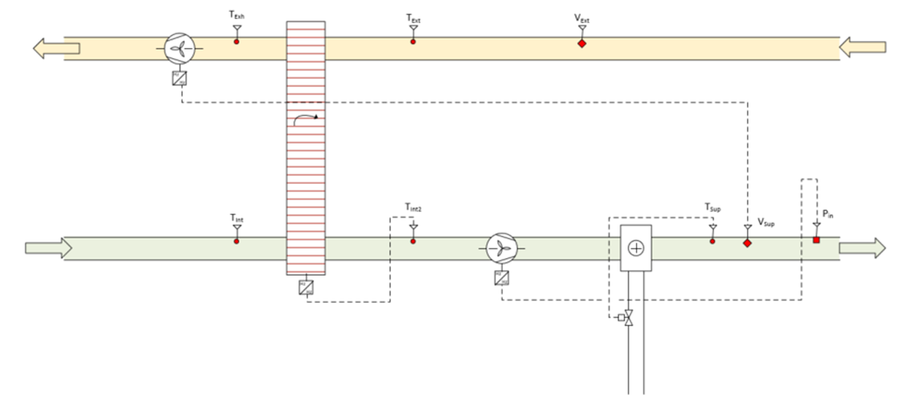
Figure 1: Principle ventilation flow sheet

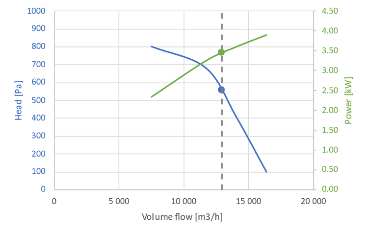
Figure 2: Fan characteristics

The supply of air to the zones is controlled by individual dampers. The dampers are controlled to keep the CO₂ level below the threshold. Default is 800 ppm.

Hydronic heating system

The layout of the hydronic heating system is shown in Figure 3. Piping segments are modeled between the main distribution pipes and the control valves for both the ventilation and radiator circuits.

Heat is supplied by a district heating system. The temperature of the district heating is fixed to 65 °C. The supply temperature of the hydronic heating system is controlled by the flow on the primary side of the district heating heat exchanger. The setpoint follows the outdoor temperature compensation curve shown in Figure 4.

The main circulation pump sustains a fixed pressure lift. The baseline setpoint is 35 kPa. This is also the maximum possible pressure difference of the pump.

The control valve of the radiator regulates after the measured indoor temperature. The baseline controller implements fixed setpoint of 22 °C.

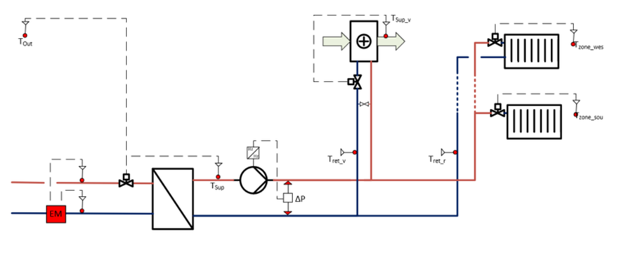
Figure 3: Principle hydronic flow sheet

The design specifications of the heat exchangers are given in Table 1.

Table 1: Design specification of heat exchangers

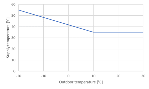
Figure 4: Baseline controller outdoor temperature compensation curve

Additional systems

An automatic shading system has been added. The shading is automatically activated if the solar irradiation on the façade is above 150 W/m². The position of the shading (0-1) can be directly overwritten through the API

Important modeling assumptions

• Model covers only one floor with offices. Adiabatic connection to floors above and below
• Single radiator representing all radiators in each zone.
• Constant infiltration rate of 0.2 air changes per hour. In addition, comes eventual mismatch between supply and extract flow rates in the AHU.

Emulator I/O’s

Inputs

Below are listed possible inputs from the external controller model to the emulator model.

Outputs

Below are listed the available outputs from the emulator.

Forecasts

The following forecast parameters are available from the emulator:

Energy prices

Electricity and district heating h the same dynamic price signal. The energy price is based on historic electricity spot market prices, corresponding to the climate data in the emulator. More details on this can be found in the general competition description.

Rules

To ensure that the competition is conducted in a fair and ethical manner, and that all participants should hold to a high standard of conduct:

• Respect: Participants are expected to treat others with respect, regardless of their background, identity, or affiliation.
• Honesty: Participants are expected to be honest and truthful in their submissions, and not to plagiarize or copy the work of others.
• Integrity: Participants are expected to maintain the integrity of the competition and not engage in any activity that could compromise the fairness or accuracy of the results.
• Confidentiality: Participants are expected to keep the data provided for the competition confidential and not to share it with others.
• Legal Compliance: Participants are expected to comply with all applicable laws, regulations, and ethical standards.
• Consequences: Violations of the Code of Conduct may result in disqualification or other sanctions, as determined by the competition organizers.

Sponsors

AES Innovation (Turkey), Akademiska Hus (Sweden), Kiona (Norway), ReMoni (Denmark), SYNAVISION GmbH (Germany)